Als Beispiel für unsupervised learning schauen wir uns den ML-Algorithmus k-means an. Der Algorithmus unterteilt Merkmalsvektoren in k Klassen (sogenannte Cluster).

Algorithmus

1. Wähle zufällig k Punkte, sogenannte Clusterzentren (clustroids)
2. Ordne jeden Punkt dem nächsten Clusterzentrum zu
3. Berechne neue Clusterzentren als Gravitationsmittelpunkt jedes Clusters
4. Wiederhole Schritte 2 und 3

Struktogram k-means

Beispiel

Wir schauen uns den Algorithmus an folgendem Beispiel an und beziehen uns dabei auf die oben genannten 4 Schritte:

Ausgangslage
Die grau eingetragenen Punkte sollen in 3 Cluster unterteilt werden.

Schritt 1
Es werden zufällig drei Clusterzentren gewählt.
(in der Abbildung farbig hervorgehoben)
Alternativ könnte man auch 3 vorhandene Punkte als Clusterzentrum auswählen.

Schritt 2
Alle Punkte werden ihrem nächsten Clusterzentrum zugeordnet: es entstehen 3 Cluster.
(in der Abbildung farbig hervorgehoben)

Schritt 3
Für jeden Cluster wird das Gravitationszentrum berechnet. Anschliessend wird das Clusterzentrum auf das Gravitationszentrum gesetzt.

Wiederholung
Die Schritte 2 und 3 werden mehrmals wiederholt. Die Clusterzentren verschieben sich dabei immer weniger.
Am Schluss erhalten wir die gewünschten 3 Cluster.

Aufgabe: Endzustand

Überlege dir, wie die 3 Cluster am Schluss aussehen würden, wenn man die Schritte 2 und 3 noch mindestens 5 Mal wiederholt

Python

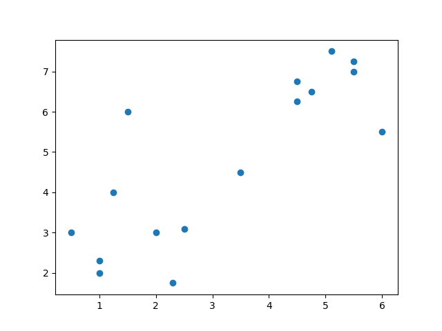
Wir verwenden wiederum die Werte von Heinz-Willhelms Pilzmaschine, entfernen aber die Labels und nehmen die beiden später gefundenen Pilze gleich dazu. Unsere Punkte sind wie folgt angeordnet und sollen in 2 Cluster unterteilt werden.

Zu kategorisierende Punkte

import matplotlib.pyplot as plt
from sklearn.cluster import KMeans

data = [
    (1, 2),
    (0.5, 3),
    (1.25, 4),
    (2.3, 1.75),
    (1, 2.3),
    (2.5, 3.1),
    (1.5, 6),
    (5.5, 7),
    (6, 5.5),
    (5.5, 7.25),
    (4.5, 6.75),
    (4.5, 6.25),
    (4.75, 6.5),
    (5.1, 7.5),
    (2, 3),
    (3.5, 4.5)
]

x_points = [point[0] for point in data]
y_points = [point[1] for point in data]

plt.scatter(x_points, y_points)

plt.show()
plt.close()

Aufgabe: a oder b?

Gehe vom obenstehenden Beispiel aus und versuche, diese Daten in 2 Cluster zu unterteilen.

1. du löst das Ganze selbst, indem du eigene Funktionen zur Clusterzentren-Berechnung und Cluster-Bildung definierst
2. du verwendest KMeans aus dem Paket sklearn.cluster

mehr: Tipp zu Teilaufgabe b

KMeans kann wie folgt aufgerufen werden:

from sklearn.cluster import KMeans
...
kmeans = KMeans(n_clusters=2, init='k-means++', max_iter=300, n_init=10, random_state=0)
y_kmeans = kmeans.fit_predict(data)

bleibt noch die Interpretation des Resultats y_kmeans. Schön wäre, wenn wir die Punkte wirklich farbig darstellen können!

Lösung

a) eigene Lösung

import matplotlib.pyplot as plt
import random

class Vector:
    def __init__(self, x, y):
        self.x = x
        self.y = y
        self.color = "black"

    def setColor(self, color):
        self.color = color


class Cluster(Vector):
    def __init__(self, point):
        super().__init__(point.x, point.y)
        self.points = []

    def distance(self, point):
        dx = self.x - point.x
        dy = self.y - point.y
        return (dx**2 + dy**2)**0.5

    def clearPoints(self):
        self.points = []

    def addPoint(self, point):
        self.points.append(point)
    
    def setColor(self, color):
        super().setColor(color)
        for point in self.points:
            point.setColor(color)

    def calculateMeans(self):
        x_mean = 0
        y_mean = 0
        n = len(self.points)
        for point in self.points:
            x_mean += point.x
            y_mean += point.y
        self.x = x_mean / n
        self.y = y_mean / n

    def __str__(self):
        return f"Center ({self.x}/{self.y}), Points: {self.points}"


class Algorithm():
    def __init__(self, clusters=3, iterations=10,colors=[]):
        self.n_clusters = clusters
        self.iterations = iterations
        self.colors = colors

    def setPoints(self, points):
        self.points = points

    def getXPoints(self):
        return [point.x for point in self.points]

    def getColors(self):
        return [point.color for point in self.points]

    def getYPoints(self):
        return [point.y for point in self.points]

    def makeClusters(self):
        # Zufällige Punkte für Cluster auswählen
        center_idx = random.sample(range(0, len(self.points)), self.n_clusters)
        # Cluster erstellen
        self.clusters = [Cluster(self.points[idx]) for idx in center_idx]

        self.assignPoints()
        for i in range(self.iterations):
            for cluster in self.clusters:
                cluster.calculateMeans()
                self.assignPoints()

        for i in range(len(self.clusters)):
            self.clusters[i].setColor(self.colors[i])

    def assignPoints(self):
        for cluster in self.clusters:
            cluster.clearPoints()
        # Für jeden Punkt Distanz zu Cluter berechnen
        for point in self.points:
            distances = [cluster.distance(point) for cluster in self.clusters]
            idx = distances.index(min(distances))
            self.clusters[idx].addPoint(point)


data = [
    Vector(1, 2),
    Vector(0.5, 3),
    Vector(1.25, 4),
    Vector(2.3, 1.75),
    Vector(1, 2.3),
    Vector(2.5, 3.1),
    Vector(1.5, 6),
    Vector(5.5, 7),
    Vector(6, 5.5),
    Vector(5.5, 7.25),
    Vector(4.5, 6.75),
    Vector(4.5, 6.25),
    Vector(4.75, 6.5),
    Vector(5.1, 7.5),
    Vector(2, 3),
    Vector(3.5, 4.5)
]

alg = Algorithm(
    clusters=3,
    iterations=20,
    colors = ["red","green","blue","yellow","orange"]
)
alg.setPoints(data)
alg.makeClusters()

plt.scatter(alg.getXPoints(), alg.getYPoints(), color=alg.getColors())

plt.show()
plt.close()

b) mit sklearn

import matplotlib.pyplot as plt
from sklearn.cluster import KMeans

data = [
    (1, 2),
    (0.5, 3),
    (1.25, 4),
    (2.3, 1.75),
    (1, 2.3),
    (2.5, 3.1),
    (1.5, 6),
    (5.5, 7),
    (6, 5.5),
    (5.5, 7.25),
    (4.5, 6.75),
    (4.5, 6.25),
    (4.75, 6.5),
    (5.1, 7.5),
    (2, 3),
    (3.5, 4.5)
]

x_points = [point[0] for point in data]
y_points = [point[1] for point in data]

kmeans = KMeans(n_clusters=2, init='k-means++', max_iter=300, n_init=10, random_state=0)
y_kmeans = kmeans.fit_predict(data)

print(y_kmeans)

palette = ["red", "green", "blue", "yellow"]
colors = [palette[i] for i in y_kmeans]

plt.scatter(x_points, y_points, color=colors)

plt.show()
plt.close()

Iris-Dataset

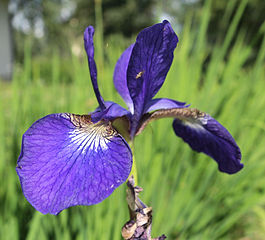
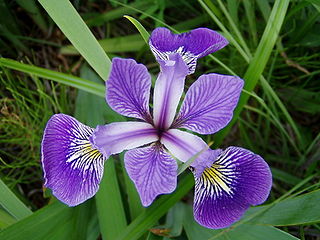
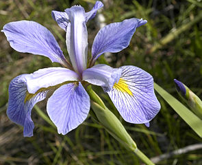
Für den sogenannten Iris-Datensatz wurden von 3 verschiedenen Schwertlilien-Arten je 50 Exemplare ausgemessen. Die Messerwert sind Länge und Breite des Kelchblatt (sepal) sowie Länge und Breite des Blütenblatts (petal).

Iris setosa^[1]

Iris versicolor^[2]

Iris virginica ^[3]

Der Datensatz liegt im CSV-Format vor:

"sepal.length","sepal.width","petal.length","petal.width","variety"
5.1,3.5,1.4,.2,"Setosa"
4.9,3,1.4,.2,"Setosa"
4.7,3.2,1.3,.2,"Setosa"
4.6,3.1,1.5,.2,"Setosa"
5,3.6,1.4,.2,"Setosa"
5.4,3.9,1.7,.4,"Setosa"
4.6,3.4,1.4,.3,"Setosa"
5,3.4,1.5,.2,"Setosa"
4.4,2.9,1.4,.2,"Setosa"
4.9,3.1,1.5,.1,"Setosa"
5.4,3.7,1.5,.2,"Setosa"
4.8,3.4,1.6,.2,"Setosa"
4.8,3,1.4,.1,"Setosa"
4.3,3,1.1,.1,"Setosa"
5.8,4,1.2,.2,"Setosa"
5.7,4.4,1.5,.4,"Setosa"
5.4,3.9,1.3,.4,"Setosa"
5.1,3.5,1.4,.3,"Setosa"
5.7,3.8,1.7,.3,"Setosa"
5.1,3.8,1.5,.3,"Setosa"
5.4,3.4,1.7,.2,"Setosa"
5.1,3.7,1.5,.4,"Setosa"
4.6,3.6,1,.2,"Setosa"
5.1,3.3,1.7,.5,"Setosa"
4.8,3.4,1.9,.2,"Setosa"
5,3,1.6,.2,"Setosa"
5,3.4,1.6,.4,"Setosa"
5.2,3.5,1.5,.2,"Setosa"
5.2,3.4,1.4,.2,"Setosa"
4.7,3.2,1.6,.2,"Setosa"
4.8,3.1,1.6,.2,"Setosa"
5.4,3.4,1.5,.4,"Setosa"
5.2,4.1,1.5,.1,"Setosa"
5.5,4.2,1.4,.2,"Setosa"
4.9,3.1,1.5,.2,"Setosa"
5,3.2,1.2,.2,"Setosa"
5.5,3.5,1.3,.2,"Setosa"
4.9,3.6,1.4,.1,"Setosa"
4.4,3,1.3,.2,"Setosa"
5.1,3.4,1.5,.2,"Setosa"
5,3.5,1.3,.3,"Setosa"
4.5,2.3,1.3,.3,"Setosa"
4.4,3.2,1.3,.2,"Setosa"
5,3.5,1.6,.6,"Setosa"
5.1,3.8,1.9,.4,"Setosa"
4.8,3,1.4,.3,"Setosa"
5.1,3.8,1.6,.2,"Setosa"
4.6,3.2,1.4,.2,"Setosa"
5.3,3.7,1.5,.2,"Setosa"
5,3.3,1.4,.2,"Setosa"
7,3.2,4.7,1.4,"Versicolor"
6.4,3.2,4.5,1.5,"Versicolor"
6.9,3.1,4.9,1.5,"Versicolor"
5.5,2.3,4,1.3,"Versicolor"
6.5,2.8,4.6,1.5,"Versicolor"
5.7,2.8,4.5,1.3,"Versicolor"
6.3,3.3,4.7,1.6,"Versicolor"
4.9,2.4,3.3,1,"Versicolor"
6.6,2.9,4.6,1.3,"Versicolor"
5.2,2.7,3.9,1.4,"Versicolor"
5,2,3.5,1,"Versicolor"
5.9,3,4.2,1.5,"Versicolor"
6,2.2,4,1,"Versicolor"
6.1,2.9,4.7,1.4,"Versicolor"
5.6,2.9,3.6,1.3,"Versicolor"
6.7,3.1,4.4,1.4,"Versicolor"
5.6,3,4.5,1.5,"Versicolor"
5.8,2.7,4.1,1,"Versicolor"
6.2,2.2,4.5,1.5,"Versicolor"
5.6,2.5,3.9,1.1,"Versicolor"
5.9,3.2,4.8,1.8,"Versicolor"
6.1,2.8,4,1.3,"Versicolor"
6.3,2.5,4.9,1.5,"Versicolor"
6.1,2.8,4.7,1.2,"Versicolor"
6.4,2.9,4.3,1.3,"Versicolor"
6.6,3,4.4,1.4,"Versicolor"
6.8,2.8,4.8,1.4,"Versicolor"
6.7,3,5,1.7,"Versicolor"
6,2.9,4.5,1.5,"Versicolor"
5.7,2.6,3.5,1,"Versicolor"
5.5,2.4,3.8,1.1,"Versicolor"
5.5,2.4,3.7,1,"Versicolor"
5.8,2.7,3.9,1.2,"Versicolor"
6,2.7,5.1,1.6,"Versicolor"
5.4,3,4.5,1.5,"Versicolor"
6,3.4,4.5,1.6,"Versicolor"
6.7,3.1,4.7,1.5,"Versicolor"
6.3,2.3,4.4,1.3,"Versicolor"
5.6,3,4.1,1.3,"Versicolor"
5.5,2.5,4,1.3,"Versicolor"
5.5,2.6,4.4,1.2,"Versicolor"
6.1,3,4.6,1.4,"Versicolor"
5.8,2.6,4,1.2,"Versicolor"
5,2.3,3.3,1,"Versicolor"
5.6,2.7,4.2,1.3,"Versicolor"
5.7,3,4.2,1.2,"Versicolor"
5.7,2.9,4.2,1.3,"Versicolor"
6.2,2.9,4.3,1.3,"Versicolor"
5.1,2.5,3,1.1,"Versicolor"
5.7,2.8,4.1,1.3,"Versicolor"
6.3,3.3,6,2.5,"Virginica"
5.8,2.7,5.1,1.9,"Virginica"
7.1,3,5.9,2.1,"Virginica"
6.3,2.9,5.6,1.8,"Virginica"
6.5,3,5.8,2.2,"Virginica"
7.6,3,6.6,2.1,"Virginica"
4.9,2.5,4.5,1.7,"Virginica"
7.3,2.9,6.3,1.8,"Virginica"
6.7,2.5,5.8,1.8,"Virginica"
7.2,3.6,6.1,2.5,"Virginica"
6.5,3.2,5.1,2,"Virginica"
6.4,2.7,5.3,1.9,"Virginica"
6.8,3,5.5,2.1,"Virginica"
5.7,2.5,5,2,"Virginica"
5.8,2.8,5.1,2.4,"Virginica"
6.4,3.2,5.3,2.3,"Virginica"
6.5,3,5.5,1.8,"Virginica"
7.7,3.8,6.7,2.2,"Virginica"
7.7,2.6,6.9,2.3,"Virginica"
6,2.2,5,1.5,"Virginica"
6.9,3.2,5.7,2.3,"Virginica"
5.6,2.8,4.9,2,"Virginica"
7.7,2.8,6.7,2,"Virginica"
6.3,2.7,4.9,1.8,"Virginica"
6.7,3.3,5.7,2.1,"Virginica"
7.2,3.2,6,1.8,"Virginica"
6.2,2.8,4.8,1.8,"Virginica"
6.1,3,4.9,1.8,"Virginica"
6.4,2.8,5.6,2.1,"Virginica"
7.2,3,5.8,1.6,"Virginica"
7.4,2.8,6.1,1.9,"Virginica"
7.9,3.8,6.4,2,"Virginica"
6.4,2.8,5.6,2.2,"Virginica"
6.3,2.8,5.1,1.5,"Virginica"
6.1,2.6,5.6,1.4,"Virginica"
7.7,3,6.1,2.3,"Virginica"
6.3,3.4,5.6,2.4,"Virginica"
6.4,3.1,5.5,1.8,"Virginica"
6,3,4.8,1.8,"Virginica"
6.9,3.1,5.4,2.1,"Virginica"
6.7,3.1,5.6,2.4,"Virginica"
6.9,3.1,5.1,2.3,"Virginica"
5.8,2.7,5.1,1.9,"Virginica"
6.8,3.2,5.9,2.3,"Virginica"
6.7,3.3,5.7,2.5,"Virginica"
6.7,3,5.2,2.3,"Virginica"
6.3,2.5,5,1.9,"Virginica"
6.5,3,5.2,2,"Virginica"
6.2,3.4,5.4,2.3,"Virginica"
5.9,3,5.1,1.8,"Virginica"

Das CSV-Format (comma-separated-values) enthält durch Komma-getrennte Datensätze (zeilenweise). Die ersten 4 Einträge sähen in Tabellenform wie folgt aus:

sepal.length	sepal.width	petal.length	petal.width	variety
5.1	3.5	1.4	.2	Setosa
4.9	3	1.4	.2	Setosa
4.7	3.2	1.3	.2	Setosa
4.6	3.1	1.5	.2	Setosa

Die Datei lässt sich hier runterladen:

iris.csv

Die Python-Library pandas eignet sich, um Daten aus externen Dateien zu lesen. Das folgende Skript liest die Datei iris.csv (muss im selben Verzeichnis liegen wie das Skript) und extrahiert daraus die Spalten mit den Merkmalen sowie diejenige mit den Labels.

import pandas as pd

iris = pd.read_csv('iris.csv')
X = iris[["sepal.length", "sepal.width", "petal.length", "petal.width"]].values
y = iris["variety"].values

Aufgabe

Schaffst du es, das Iris-Datenset in 3 Cluster zu unterteilen? Wenn ja, passen die Cluster mit den Arten überein?

---

1. Tiia Monto via Wikimedia Commons, CC BY-SA 4.0 ↩︎

2. unknown via Wikimedia Commons, CC BY-SA 3.0 ↩︎

3. Frank Mayfield via Wikimedia Commons, CC BY-SA 2.0 ↩︎